While analysing the data acquired by testing the prototype with and without the filter we came to the conclusion that the filter was not perfect for our situation.
Hypothetically an ideal filter would be cutting of the majority of the excitation light and letting it pass through 100% of the emitted green light. Under these conditions, the count difference measured between two time points in one sample should only come from the increase in fluorescence, with or without a filter. If we measure without a filter at two different time points, we will measure the scattered light and the fluorescence. At the next time point we expect the fluorescence to have increased and no the scattered light, which will amount to a count difference because of the increase of the fluorescence. When testing with a filter, the difference between the count at the 2 time points will come from the increase of fluorescence only and the difference between the two time points should be the same as in the measurements without filter.
Here we show the graphs of the relative fluorescence (divided by absorbance) with and without filter, measured at two different time points.

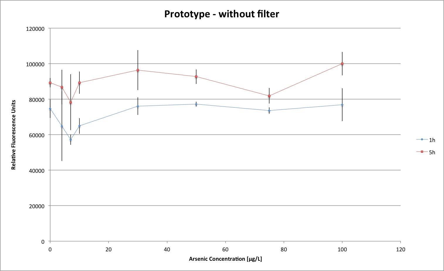
We can see that the difference measured between 2 time points of the same sample in the 2 graphs differs by 5 fold between the 2 data sets, which means that the filter is not exactly what we want it to be.
What we need to do know is analyse the spectra of our excitation LED, emission light and filter to be able to predict what we will be measuring at the sensor.
